1. Generate makefile by cmake
cmake -G "MSYS Makefiles" -DBUILD_SHARED_LIBS=ON
In msys bash do follows
2. Compile in mingw
make
which would generate dll library XXX.dll
3. Generate def file
gendef XXX.dll
In VS command prompt do follows
4. Generate MSVC library
lib /machines:x64 /def:XXX.def /out:XXX.lib
A MSVC dll file could also be transfered into mingw .a file
1. Generate def file
gendef XXX.dll
2. Generate .a library
dlltool --dllname XXX.dll --input-def XXX.def --output-lib libXXX.a

FEM as a tool of PDE solver and its open source implementation
1. Finite element function space
Once a domain Ω has been partitioned into cells, one may define a local function space V on each
cell Ti and use these local function spaces to build the global function space Vh. A cell Ti together
with a local function space V and a set of rules for describing the functions in V is called a finite
element. This definition reads as follows: a finite element is a triple (T, V, L), where
• the domain T is a bounded, closed subset of $R^d$(for d = 1, 2, 3, . . . ) with nonempty interior and
piecewise smooth boundary;
• the space V = V(T) is a finite dimensional function space on T of dimension n;
• the set of degrees of freedom (nodes) L = { 1, 2,..., n} is a basis for the dual space $\hat{V}$; that
is, the space of bounded linear functionals on V.
If finite element spaces for grad, div, and curl are implemented, most types of PDEs are solvable.
• H1Space - the most common FE space of continuous, piecewise-polynomial function:
$H^1(\Omega) = \{v\in L^2(\Omega); \nabla u\in[L^2(\Omega)]^2\}$
2. Weak form of PDE
We consider a general linear variational problem written in the following canonical form: find u ∈ V such that
$a(u,v)=L(v): \forall v \in \hat{V}$
where the test space $\hat{V}$ is defined by
$\hat{V}=\{v \in H^1(\Omega):v=0\ on\ \Gamma_\Omega\}$
and the trial space V contains members of Vˆ shifted by the Dirichlet condition:
$V=\{v \in H^1(\Omega):v=u_0\ on\ \Gamma_\Omega\}$
We thus express the variational problem in terms of a bilinear form a and a linear form (functional) L:
$a: V \times \hat{V} \to R$
$L: \hat{V} \to R$
The basic idea of FEM consists of approximating the big Hilbert space $H_0^1$, e.g., by some appropriate finite-dimensional space $H_h$, where h is a positive parameter, satisfying the following conditions:
• $H_h \subseteq H_0^1$
• Solve $a(u_h,v_h)=L(v_h)$ obtain a solution $v_h$ and
• $H_h \to H_0^1 \ as \ h \to 0$
Example: Poisson problem
Find u such that
$-\Delta u=f, x \in \Omega\subset R^d$
$u=0 \ on \ \partial\Omega$
After integrating by part, we obtains its weak form
$Find \ u \in V=H^1_0(\Omega): \{v=0 \ on \ \partial\Omega\}$
$such \ that \int_\Omega\nabla u\cdot \nabla vd\Omega=\int_\Omega fvd\Omega, \forall v\in V$
where $a(u,v)=\int_\Omega\nabla u\cdot \nabla vd\Omega$, $L(v)=\int_\Omega fvd\Omega$
3. Implementation on some mathmatically oriented open source FEM software
The general FEM system could be thought of as having form $a(u_h,v_h)=L(v_h)$ and solved by following steps
3.3 Feel++
Following c++ program construct a solver for Poisson equation
auto mesh = ... // build a mesh auto Vh = Pch<a>(mesh) // define FE space auto a = form2(_trial=Vh, _test=Vh) // declare a two form //$a(u,v)=\int_\Omega\nabla u\cdot \nabla vd\Omega$
a.solve(_solution=u, _rhs=l ) // solve it
3.4 GetDP
The input file to solve Poisson equation look like:
FunctionSpace {
{ Name H1; Type Form0;
BasisFunction {
{ Name sn; NameOfCoef vn; Function BF_Node; Support D; Entity NodesOf[All]; }
}
}
}
Formulation{
{ Name Poisson; Type FemEquation;
Quantity {
{ Name v; Type Local; NameOfSpace H1; }
}
Equation {
Integral { [ a[] * Dof{d v}, {d v} ] ; In D; Jacobian V; Integration I; }
Integral { [ f[], {v} ] ; In D; Jacobian V; Integration I; }
}
}
}
3.5 Sundance As a part of big Trilinos, it seems that it is not on develop right now. Compile error may happen due to its old-styled code. A modified fork is given here.
// get a mesh Mesh mesh = meshSrc.getMesh(); /* Test and unknown function */
BasisFamily basis = new Lagrange(1);
Expr u = new UnknownFunction(basis, "u");
Expr v = new TestFunction(basis, "v"); /* We need a quadrature rule for doing the integrations */
QuadratureFamily quad1 = new GaussianQuadrature(1);
/** Write the weak form */
Expr eqn
= Integral(interior, (grad*u)*(grad*v), quad1)
+ Integral(east, v, quad1); /* Set up linear problem */
LinearProblem prob(mesh, eqn, bc, v, u, vecType);
/* --- solve the problem --- */
/* Create the solver as specified by parameters in an XML file */
LinearSolver<double> solver
= LinearSolverBuilder::createSolver(solverFile);
/* Solve! The solution is returned as an Expr containing a
* DiscreteFunction */
Expr soln = prob.solve(solver); 3.6 MFEM You cannot define above two form and one form youeself, MFEM provides prepared classes of one form and two form integrators instead. Something like, e.g.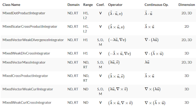
Therefore, it is not that strictly mathematically oriented than above ones but would expect more computational efficiency because software intepretation of one form, two form definition are not needed anymore.
Its implementation on Poisson problem looks like:
// read a mesh
Mesh *mesh = new Mesh(mesh_file, 1, 1);
// define FE space
FiniteElementCollection *fec;
FiniteElementSpace *fespace = new FiniteElementSpace(mesh, fec);
// define one form
LinearForm *b = new LinearForm(fespace);
ConstantCoefficient one(1.0);
b->AddDomainIntegrator(new DomainLFIntegrator(one));
b->Assemble();
// define two form
BilinearForm *a = new BilinearForm(fespace);
a->AddDomainIntegrator(new MixedGradGradIntegrator(one));
a->Assemble();
Reference:
1) A Logg, K-A Mardel. GN Wells: Automated Solution of Differential Equations by the Finite Element Method, Springer-Verlag. 2012
2) Eric Sonnendru¨cker, Ahmed Ratnani : Advanced Finite Element Methods
The construction of the finite element space Vh begins with subdividing the domain $\Omega$ into a set of non-overlapping or overlapping, such as those implemented in GFEM, cells $T_1,T_2,...T_m$. The domain $\Omega$ can now be approximated with a mesh domain,
$T_h(\Omega)=\cup{T_i}$
The cells are typically simple polygonal shapes like intervals, triangles, quadrilaterals, tetrahedra or hexahedra but also could be described by B-splines as in isogeometric analysis.
cell Ti and use these local function spaces to build the global function space Vh. A cell Ti together
with a local function space V and a set of rules for describing the functions in V is called a finite
element. This definition reads as follows: a finite element is a triple (T, V, L), where
• the domain T is a bounded, closed subset of $R^d$(for d = 1, 2, 3, . . . ) with nonempty interior and
piecewise smooth boundary;
• the space V = V(T) is a finite dimensional function space on T of dimension n;
• the set of degrees of freedom (nodes) L = { 1, 2,..., n} is a basis for the dual space $\hat{V}$; that
is, the space of bounded linear functionals on V.
If finite element spaces for grad, div, and curl are implemented, most types of PDEs are solvable.
• H1Space - the most common FE space of continuous, piecewise-polynomial function:
$H^1(\Omega) = \{v\in L^2(\Omega); \nabla u\in[L^2(\Omega)]^2\}$
• HCurlSpace - FE space of vector-valued functions discontinuous along mesh edges, with continunous tangential component on the edges
$H(curl,\Omega) = \{E\in [L^2(\Omega)]^2; \nabla\times E\in L^2(\Omega)\}$
• HDivSpace - FE space of vector-valued functions discontinuous along mesh edges, with continunous normal component on the edges
$H(div,\Omega) = \{v\in [L^2(\Omega)]^2; \nabla\cdot v\in L^2(\Omega)\}$
We consider a general linear variational problem written in the following canonical form: find u ∈ V such that
$a(u,v)=L(v): \forall v \in \hat{V}$
where the test space $\hat{V}$ is defined by
$\hat{V}=\{v \in H^1(\Omega):v=0\ on\ \Gamma_\Omega\}$
and the trial space V contains members of Vˆ shifted by the Dirichlet condition:
$V=\{v \in H^1(\Omega):v=u_0\ on\ \Gamma_\Omega\}$
We thus express the variational problem in terms of a bilinear form a and a linear form (functional) L:
$a: V \times \hat{V} \to R$
$L: \hat{V} \to R$
The basic idea of FEM consists of approximating the big Hilbert space $H_0^1$, e.g., by some appropriate finite-dimensional space $H_h$, where h is a positive parameter, satisfying the following conditions:
• $H_h \subseteq H_0^1$
• Solve $a(u_h,v_h)=L(v_h)$ obtain a solution $v_h$ and
• $H_h \to H_0^1 \ as \ h \to 0$
Example: Poisson problem
Find u such that
$-\Delta u=f, x \in \Omega\subset R^d$
$u=0 \ on \ \partial\Omega$
After integrating by part, we obtains its weak form
$Find \ u \in V=H^1_0(\Omega): \{v=0 \ on \ \partial\Omega\}$
$such \ that \int_\Omega\nabla u\cdot \nabla vd\Omega=\int_\Omega fvd\Omega, \forall v\in V$
where $a(u,v)=\int_\Omega\nabla u\cdot \nabla vd\Omega$, $L(v)=\int_\Omega fvd\Omega$
3. Implementation on some mathmatically oriented open source FEM software
The general FEM system could be thought of as having form $a(u_h,v_h)=L(v_h)$ and solved by following steps
• Build a mesh Th. It could be also read from exsting mesh files.
• Define the finite element space Vh
• Define the finite element space Vh
• Define the variational problem P $a(u_h,v_h)=L(v_h)$
• Solve the problem P
• Postprocess
Lets see how it is really implemented in some open source FEM softwares
3.1 freeFEM++
We need prepare following input file:
mesh Th=square(10,10) // generate a mesh Th
fespace Vh(Th,P1) // define FE space Vh on Th by element type P1
Vh u,v // declear funtion in Vh
func f = -1 // constant function
func g =0 // constant function
// $a(u,v)=\int_\Omega\nabla u\cdot \nabla vd\Omega$
problem Poisson(u,v) = int2d(Th)(dx(uh)*dx(vh)+dy(uh)*dy(vh))
-int2d(f*v) // $L(v)=\int_\Omega fvd\Omega$
+on(C, g) // u=g on boundary C
Poisson // solve it
plot(u) // visualize solution
3.2 FEniCS
Following python script is needed:
from fenics import *
Th = UnitSquareMesh(10, 10) // generate a mesh Th
Vh = FunctionSpace(mesh, ’P’, 1) // define FE space Vh on Th by element type P1
Vh = FunctionSpace(mesh, ’P’, 1) // define FE space Vh on Th by element type P1
u = TrialFunction(Vh) // declear funtion in Vh
v = TestFunction(Vh) // declear funtion in Vh
v = TestFunction(Vh) // declear funtion in Vh
f = Constant(-1.0) // constant function
g = Constant(0.0) // constant
a = dot(grad(u), grad(v))*dx // $a(u,v)=\int_\Omega\nabla u\cdot \nabla vd\Omega$
L = f*v*dx // $L(v)=\int_\Omega fvd\Omega$
L = f*v*dx // $L(v)=\int_\Omega fvd\Omega$
def boundary(x, on_boundary):
return on_boundary
bc = DirichletBC(V, g, boundary)
return on_boundary
bc = DirichletBC(V, g, boundary)
solve(a == L, u, bc) // solve it
plot(u) // visualize solution
A Julia wrapper of FEniCS given here.
3.3 Feel++
Following c++ program construct a solver for Poisson equation
auto mesh = ... // build a mesh auto Vh = Pch<a>(mesh) // define FE space auto a = form2(_trial=Vh, _test=Vh) // declare a two form //$a(u,v)=\int_\Omega\nabla u\cdot \nabla vd\Omega$
a.solve(_solution=u, _rhs=l ) // solve it
3.4 GetDP
The input file to solve Poisson equation look like:
FunctionSpace {
{ Name H1; Type Form0;
BasisFunction {
{ Name sn; NameOfCoef vn; Function BF_Node; Support D; Entity NodesOf[All]; }
}
}
}
Formulation{
{ Name Poisson; Type FemEquation;
Quantity {
{ Name v; Type Local; NameOfSpace H1; }
}
Equation {
Integral { [ a[] * Dof{d v}, {d v} ] ; In D; Jacobian V; Integration I; }
Integral { [ f[], {v} ] ; In D; Jacobian V; Integration I; }
}
}
}
3.5 Sundance As a part of big Trilinos, it seems that it is not on develop right now. Compile error may happen due to its old-styled code. A modified fork is given here.
// get a mesh Mesh mesh = meshSrc.getMesh(); /* Test and unknown function */
BasisFamily basis = new Lagrange(1);
Expr u = new UnknownFunction(basis, "u");
Expr v = new TestFunction(basis, "v"); /* We need a quadrature rule for doing the integrations */
QuadratureFamily quad1 = new GaussianQuadrature(1);
/** Write the weak form */
Expr eqn
= Integral(interior, (grad*u)*(grad*v), quad1)
+ Integral(east, v, quad1); /* Set up linear problem */
LinearProblem prob(mesh, eqn, bc, v, u, vecType);
/* --- solve the problem --- */
/* Create the solver as specified by parameters in an XML file */
LinearSolver<double> solver
= LinearSolverBuilder::createSolver(solverFile);
* DiscreteFunction */
Expr soln = prob.solve(solver); 3.6 MFEM You cannot define above two form and one form youeself, MFEM provides prepared classes of one form and two form integrators instead. Something like, e.g.

Therefore, it is not that strictly mathematically oriented than above ones but would expect more computational efficiency because software intepretation of one form, two form definition are not needed anymore.
Its implementation on Poisson problem looks like:
// read a mesh
Mesh *mesh = new Mesh(mesh_file, 1, 1);
// define FE space
FiniteElementCollection *fec;
FiniteElementSpace *fespace = new FiniteElementSpace(mesh, fec);
// define one form
LinearForm *b = new LinearForm(fespace);
ConstantCoefficient one(1.0);
b->AddDomainIntegrator(new DomainLFIntegrator(one));
b->Assemble();
// define two form
BilinearForm *a = new BilinearForm(fespace);
a->AddDomainIntegrator(new MixedGradGradIntegrator(one));
a->Assemble();
Reference:
1) A Logg, K-A Mardel. GN Wells: Automated Solution of Differential Equations by the Finite Element Method, Springer-Verlag. 2012
2) Eric Sonnendru¨cker, Ahmed Ratnani : Advanced Finite Element Methods
吃饭论法
最近日本出现了一个新词汇"ご飯論法", 用来描述政治家的国会答辩。看之不禁喷饭。其原始版本出于此处。
▼Q「朝ごはんは食べなかったんですか?」A「ご飯は食べませんでした(パンは食べましたが、それは黙っておきます)」Q「何も食べなかったんですね?」A「何も、と聞かれましても、どこまでを食事の範囲に入れるかは、必ずしも明確ではありませんので…」
▼Q「では、何か食べたんですか?」A「お尋ねの趣旨が必ずしもわかりませんが、一般論で申し上げますと、朝食を摂(と)る、というのは健康のために大切であります」Q「いや、一般論を伺っているんじゃないんです。あなたが昨日、朝ごはんを食べたかどうかが、問題なんですよ」A「ですから…」
▼Q「じゃあ、聞き方を変えましょう。ご飯、白米ですね、それは食べましたか」A「そのように一つ一つのお尋ねにこたえていくことになりますと、私の食生活をすべて開示しなければならないことになりますので、それはさすがに、そこまでお答えすることは、大臣としての業務に支障をきたしますので」
------------------
译文如下
Q 吃早饭了吗
A 没吃(虽然吃了面包,但我不说)
Q 什么都没吃吗
A 这就不好说了。所谓吃饭(日语是食事)的定义原本就不明确
Q 那么你吃了些什么?
A 我不明白你问题的意思。就一般情况而言,早饭对于健康非常重要
Q 我没有问你一般性的问题,只是问你今天(原文为昨天)是否吃了早饭
A 嗯---
Q 那么,我改变一下问法。你吃了饭,也就是吃了白米吗?
A 你这样一个一个的问,意味着我的饮食生活全部都要公开,这样的话我作为大臣还怎么工作!
------------------
订阅:
博文 (Atom)
VS Code下cmake, c++编译,调试环境的构成步骤
1 下载必须extension 按[Ctrl+Shift+X]打开extension窗口,选择安装"C/C++", "CMake", "CMake Tools" 2 在VSCode下打开作业目录 ...

-
 学过连续体力学(包括固体力学,流体力学等)都知道应力张量是对称的(下面将说明它是有条件的)。 对于初学者, 这似乎有些难于理解, 如 http://forum.simwe.com/forum.php?mod=viewthread&tid=503234&hig...
 -
 1. 什么是体积锁死现象 图1 平面应变模型 在图1所示的又两个三角形单元组成的平面应变问题中,如果变形体材料是不可压缩的,那么我们不管在加载点施加多大的力,从有限元法计算得到的所有节点的所有位移都为零。因为任意位移都会导致 两个三角形中的一个的体积...
 -
假设时间步i中的所有物理量X i 已知, 如果时间步i+1中的所有物理量X i+1 可以表为X i 的显函数 (1) X i+1 = F(X i ) (注;本文以下标i,i+1等表示时间步) 则该物理量X可以显式计算。而如果 (2) ...