1. Finite element function space
The construction of the finite element space Vh begins with subdividing the domain $\Omega$ into a set of non-overlapping or overlapping, such as those implemented in GFEM, cells $T_1,T_2,...T_m$. The domain $\Omega$ can now be approximated with a mesh domain,
$T_h(\Omega)=\cup{T_i}$
The cells are typically simple polygonal shapes like intervals, triangles, quadrilaterals, tetrahedra or hexahedra but also could be described by B-splines as in isogeometric analysis.
Once a domain Ω has been partitioned into cells, one may define a local function space V on each
cell Ti and use these local function spaces to build the global function space Vh. A cell Ti together
with a local function space V and a set of rules for describing the functions in V is called a finite
element. This definition reads as follows: a finite element is a triple (T, V, L), where
• the domain T is a bounded, closed subset of $R^d$(for d = 1, 2, 3, . . . ) with nonempty interior and
piecewise smooth boundary;
• the space V = V(T) is a finite dimensional function space on T of dimension n;
• the set of degrees of freedom (nodes) L = { 1, 2,..., n} is a basis for the dual space $\hat{V}$; that
is, the space of bounded linear functionals on V.
If finite element spaces for grad, div, and curl are implemented, most types of PDEs are solvable.
• H1Space - the most common FE space of continuous, piecewise-polynomial function:
$H^1(\Omega) = \{v\in L^2(\Omega); \nabla u\in[L^2(\Omega)]^2\}$
• HCurlSpace - FE space of vector-valued functions discontinuous along mesh edges, with continunous tangential component on the edges
$H(curl,\Omega) = \{E\in [L^2(\Omega)]^2; \nabla\times E\in L^2(\Omega)\}$
• HDivSpace - FE space of vector-valued functions discontinuous along mesh edges, with continunous normal component on the edges
$H(div,\Omega) = \{v\in [L^2(\Omega)]^2; \nabla\cdot v\in L^2(\Omega)\}$
2. Weak form of PDE
We consider a general linear variational problem written in the following canonical form: find u ∈ V such that
$a(u,v)=L(v): \forall v \in \hat{V}$
where the test space $\hat{V}$ is defined by
$\hat{V}=\{v \in H^1(\Omega):v=0\ on\ \Gamma_\Omega\}$
and the trial space V contains members of Vˆ shifted by the Dirichlet condition:
$V=\{v \in H^1(\Omega):v=u_0\ on\ \Gamma_\Omega\}$
We thus express the variational problem in terms of a bilinear form a and a linear form (functional) L:
$a: V \times \hat{V} \to R$
$L: \hat{V} \to R$
The basic idea of FEM consists of approximating the big Hilbert space $H_0^1$, e.g., by some appropriate finite-dimensional space $H_h$, where h is a positive parameter, satisfying the following conditions:
• $H_h \subseteq H_0^1$
• Solve $a(u_h,v_h)=L(v_h)$ obtain a solution $v_h$ and
• $H_h \to H_0^1 \ as \ h \to 0$
Example: Poisson problem
Find u such that
$-\Delta u=f, x \in \Omega\subset R^d$
$u=0 \ on \ \partial\Omega$
After integrating by part, we obtains its weak form
$Find \ u \in V=H^1_0(\Omega): \{v=0 \ on \ \partial\Omega\}$
$such \ that \int_\Omega\nabla u\cdot \nabla vd\Omega=\int_\Omega fvd\Omega, \forall v\in V$
where
$a(u,v)=\int_\Omega\nabla u\cdot \nabla vd\Omega$, $L(v)=\int_\Omega fvd\Omega$
3. Implementation on some mathmatically oriented open source FEM software
The general FEM system could be thought of as having form
$a(u_h,v_h)=L(v_h)$ and solved by following steps
• Build a mesh Th. It could be also read from exsting mesh files.
• Define the finite element space Vh
• Define the variational problem P $a(u_h,v_h)=L(v_h)$
• Solve the problem P
• Postprocess
Lets see how it is really implemented in some open source FEM softwares
We need prepare following input file:
mesh Th=square(10,10) // generate a mesh Th
fespace Vh(Th,P1) // define FE space Vh on Th by element type P1
Vh u,v // declear funtion in Vh
func f = -1 // constant function
func g =0 // constant function
// $a(u,v)=\int_\Omega\nabla u\cdot \nabla vd\Omega$
problem Poisson(u,v) = int2d(Th)(dx(uh)*dx(vh)+dy(uh)*dy(vh))
-int2d(f*v) // $L(v)=\int_\Omega fvd\Omega$
+on(C, g) // u=g on boundary C
Poisson // solve it
plot(u) // visualize solution
Following python script is needed:
from fenics import *
Th = UnitSquareMesh(10, 10) // generate a mesh Th
Vh = FunctionSpace(mesh, ’P’, 1) // define FE space Vh on Th by element type P1
u = TrialFunction(Vh) // declear funtion in Vh
v = TestFunction(Vh) // declear funtion in Vh
f = Constant(-1.0) // constant function
g = Constant(0.0) // constant
a = dot(grad(u), grad(v))*dx // $a(u,v)=\int_\Omega\nabla u\cdot \nabla vd\Omega$
L = f*v*dx // $L(v)=\int_\Omega fvd\Omega$
def boundary(x, on_boundary):
return on_boundary
bc = DirichletBC(V, g, boundary)
solve(a == L, u, bc) // solve it
plot(u) // visualize solution
A Julia wrapper of FEniCS given
here.
3.3 Feel++
Following c++ program construct a solver for Poisson equation
auto mesh = ... // build a mesh
auto Vh = Pch<a>(mesh) // define FE space
auto a = form2(_trial=Vh, _test=Vh) // declare a two form
//$a(u,v)=\int_\Omega\nabla u\cdot \nabla vd\Omega$
a.solve(_solution=u, _rhs=l ) // solve it
3.4 GetDP
The input file to solve Poisson equation look like:
FunctionSpace {
{ Name H1; Type Form0;
BasisFunction {
{ Name sn; NameOfCoef vn; Function BF_Node; Support D; Entity NodesOf[All]; }
}
}
}
Formulation{
{ Name Poisson; Type FemEquation;
Quantity {
{ Name v; Type Local; NameOfSpace H1; }
}
Equation {
Integral { [ a[] * Dof{d v}, {d v} ] ; In D; Jacobian V; Integration I; }
Integral { [ f[], {v} ] ; In D; Jacobian V; Integration I; }
}
}
}
3.5 Sundance
As a part of big Trilinos, it seems that it is not on develop right now. Compile error may happen due to its old-styled code. A modified fork is given here.
// get a mesh
Mesh mesh = meshSrc.getMesh();
/* Test and unknown function */
BasisFamily basis = new Lagrange(1);
Expr u = new UnknownFunction(basis, "u");
Expr v = new TestFunction(basis, "v");
/* We need a quadrature rule for doing the integrations */
QuadratureFamily quad1 = new GaussianQuadrature(1);
/** Write the weak form */
Expr eqn
= Integral(interior, (grad*u)*(grad*v), quad1)
+ Integral(east, v, quad1);
/* Set up linear problem */
LinearProblem prob(mesh, eqn, bc, v, u, vecType);
/* --- solve the problem --- */
/* Create the solver as specified by parameters in an XML file */
LinearSolver<double> solver
= LinearSolverBuilder::createSolver(solverFile);
/* Solve! The solution is returned as an Expr containing a
* DiscreteFunction */
Expr soln = prob.solve(solver);
3.6 MFEM
You cannot define above two form and one form youeself, MFEM provides prepared classes of one form and two form integrators instead. Something like, e.g.
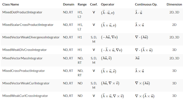
Therefore, it is not that strictly mathematically oriented than above ones but would expect more computational efficiency because software intepretation of one form, two form definition are not needed anymore.
Its implementation on Poisson problem looks like:
// read a mesh
Mesh *mesh = new Mesh(mesh_file, 1, 1);
// define FE space
FiniteElementCollection *fec;
FiniteElementSpace *fespace = new FiniteElementSpace(mesh, fec);
// define one form
LinearForm *b = new LinearForm(fespace);
ConstantCoefficient one(1.0);
b->AddDomainIntegrator(new DomainLFIntegrator(one));
b->Assemble();
// define two form
BilinearForm *a = new BilinearForm(fespace);
a->AddDomainIntegrator(new MixedGradGradIntegrator(one));
a->Assemble();
Reference:
1) A Logg, K-A Mardel. GN Wells: Automated Solution of Differential Equations by the Finite Element Method, Springer-Verlag. 2012
2) Eric Sonnendru¨cker, Ahmed Ratnani :
Advanced Finite Element Methods